How a Neural Network Learns - Step-by-Step Math with a Simple PyTorch Model

Ever wondered what really happens inside a PyTorch training loop? In this walkthrough, we break down every step — forward pass, loss, gradients, and weight updates — using a tiny neural network and simple whole-number examples. By the end, you’ll understand not just how the code runs, but how the math drives learning.

The Code

Let’s create a small model with a single linear layer of 1 neuron, with 2 input features and one output.

import torch
import torch.nn as nn
import torch.optim as optim

# data
x = torch.tensor([1, 2], dtype=float) # input with two features
y = torch.tensor([8], dtype=float) # output

model = nn.Linear(2, 1) # 2 input — 1 output

# manually set weights and bias for easy calculation
model.weight.data = torch.tensor([1, 1], dtype=float)
model.bias.data = torch.tensor([0], dtype=float)

# loss and optimizer
loss_fn = nn.MSELoss()
optimizer = optim.SGD(model.parameters(), lr=0.01)

pred = model(x)
loss = loss_fn(pred, y)
loss.backward()
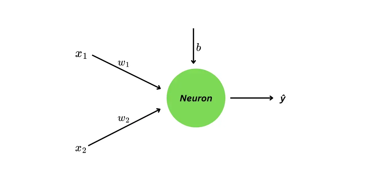
optimizer.step()

This is how the neural network looks visually.

The neural network has three parameters:

• weight $w_1$ (for feature $x_1$)
• weight $w_2$ (for feature $x_2$)
• bias $b$

We initialize them manually for easier calculation as -

$$w_1 = 1, \; w_2 = 1 \; ,\; b = 0$$

Step 1 — Forward pass (Prediction)

For the first training example:

$$\begin{gather*} x_1 = 1 \\ x_2 = 2 \\ b = 0 \\ y = 3 \end{gather*}$$

The prediction is computed using -

$$\hat{y} = w_1x_1 + w_2x_2 + b$$

Substituting the values of all variables we will get:

$$\begin{gather*} \hat{y} = 1 \cdot 1 \: + 1 \cdot 2 \: + 0 \\ \\ \hat{y} = 3 \end{gather*}$$

The model predicted 3, but the target is 8, so it’s clearly off.

Step 2 — Loss Computation

This step determines how wrong the model’s prediction is.

This is represented by function call like loss_fn(pred, y).

The first thing we measure is, the error — how far the prediction is from the true value:

$$e = \hat{y} - y$$

Errors by themselves aren’t enough for training, because we’ll have many predictions over time and we need a single number that summarizes how good or bad the model is. That number is the loss.

In this example, we are using the Mean Squared Error (MSE) loss:

$$L = \frac{1}{N} \sum_{i=1}^N \; (\hat{y}_i - y_i)^2$$

Plugging in the values, we get:

$$e = 3 - 8 = -5$$

Since $N = 1$:

$$L = (3 - 8)^2 = 25$$

The model works to reduce this loss during training.

Step 3 — Gradients (Backpropagation)

We calculate gradients when we call loss.backward().

Up to this point the model has made a prediction and we’ve calculated how wrong it is using the loss function. Now the model needs to answer a very specific question:

If I adjust each parameter just a tiny bit, will the loss go up or down — and by how much?

That “how much” is the gradient.

If you know basic calculus, this is the rate of change.

Here we will use the partial derivatives ($\partial$) since the loss $L$ depends on multiple variables at the same time ($w_1$, $w_2$ and $b$).

So we have to calculate:

$$\frac{\partial{L}}{\partial{w_1}}, \; \frac{\partial{L}}{\partial{w_2}}, \:and \; \frac{\partial{L}}{\partial{b}}$$

These tell us how sensitive the loss is to each parameter.

Let’s look at the first term, since $L$ does not directly depend on the $w_1$, we can use chain rule.

The Loss $L$ depends on error $e$, which depends on prediction $\hat{y}$, which in turns depends on the weight $w_1$. So by chain rule:

$$\frac{\partial{L}}{\partial{w_1}} = \frac{\partial{L}}{\partial{e}} \cdot \frac{\partial{e}}{\partial{\hat{y}}} \cdot \frac{\partial{\hat{y}}}{\partial{w_1}}$$

Let’s compute these terms one by one.

Derivative of $L$ w.r.t. $e$ -

$$\begin{gather*} L = e^2 \\ \\ \frac{\partial{L}}{\partial{e}} = \frac{\partial{}}{\partial{e}} (e^2) = 2e \end{gather*}$$

Derivative of $e$ w.r.t $\hat{y}$ -

$$\begin{gather*} e = \hat{y} - y \\ \\ \frac{\partial{e}}{\partial{\hat{y}}} = \frac{\partial}{\partial{\hat{y}}}(\hat{y} - y) \\ \\ \frac{\partial{e}}{\partial{\hat{y}}} = \frac{\partial{\hat{y}}}{\partial{\hat{y}}} - \frac{\partial{y}}{\partial{\hat{y}}} \\ \\ \frac{\partial{e}}{\partial{\hat{y}}} = 1 - 0 = 1 \end{gather*}$$

(Here $y$ is constant)

Derivative of $\hat{y}$ w.r.t $w_1$ -

$$\begin{gather*} \hat{y} = w_1x_1 + w_2x_2 + b \\ \\ \frac{\partial{\hat{y}}}{\partial{w_1}} = \frac{\partial{}}{\partial{w_1}} (w_1x_1 + w_2x_2 + b) \\ \\ \frac{\partial{\hat{y}}}{\partial{w_1}} = x_1 \end{gather*}$$

Here everything is a constant except the parameter $w_1$.

Final gradient for $w_1$:

$$\begin{gather*} \frac{\partial{L}}{\partial{w_1}} = \frac{\partial{L}}{\partial{e}} \cdot \frac{\partial{e}}{\partial{\hat{y}}} \cdot \frac{\partial{\hat{y}}}{\partial{w_1}} \\ \frac{\partial{L}}{\partial{w_1}} = 2e \cdot 1 \cdot x_1 = 2ex_1 \end{gather*}$$

We follow the exact same pattern for $w_2$ and $b$:

$$\begin{gather*} \frac{\partial{L}}{\partial{w_2}} = 2ex_2 \\ \\ \frac{\partial{L}}{\partial{b}} = 2e \end{gather*}$$

Plugging in numbers:

$$\begin{gather*} \frac{\partial{L}}{\partial{w_1}} = 2ex_1 = 2 \cdot (-5) \cdot 1 = -10 \\ \\ \frac{\partial{L}}{\partial{w_2}} = 2ex_2 = 2 \cdot (-5) \cdot 2 = -20 \\ \\ \frac{\partial{L}}{\partial{b}} = 2e = 2 \cdot (-5) = -10 \end{gather*}$$

Each gradient tells us how the loss reacts to each parameter.

For example, $-10$ for $w_1$ means:

If $w_1$​ increases slightly, the loss will go down by about $10$ times that amount.

Step 4: Updating parameters

The parameters are updated when calling optimizer.step().

We have computed the loss and its gradients with respect to each parameters. Now the model actually adjusts its parameters to reduce the loss.

This follows the gradient descent update rule:

$$\theta_{new} = \theta_{old} - \eta \: \cdot \: \frac{\partial{L}}{\partial{\theta}}$$

$\eta$ is the learning rate — how big a step we take in the opposite direction of the gradient.

We apply this formula to each parameter independently.

Update for $w_1$

$$\begin{gather*} (w_{1})_{new} = (w_1)_{old} - \eta \: \cdot \frac{\partial{L}}{\partial{w_1}} \\ \\ (w_{1})_{new} = 1 - 0.01 \: \cdot (-10) = 1.1 \end{gather*}$$

Update for $w_2$

$$\begin{gather*} (w_{2})_{new} = (w_2)_{old} - \eta \: \cdot \frac{\partial{L}}{\partial{w_2}} \\ \\ (w_{2})_{new} = 1 - 0.01 \: \cdot (-20) = 1.2 \\ \end{gather*}$$

Update for $b$

$$\begin{gather*} b_{new} = b_{old} - \eta \: \cdot \frac{\partial{L}}{\partial{b}} \\ \\ b_{new} = 0 - 0.01 \: \cdot (-10) = 0.1 \end{gather*}$$

Here is the summary after updates -

Parameter	Old value	Gradient	New value
$w_1$	1.0	–10	1.1
$w_2$	1.0	–20	1.2
$b$	0.0	–10	0.1

After applying gradient descent, the parameters shift slightly in the direction that reduces the loss.

I’ve also created a Jupyter Notebook with the code. Experiment with it and tweak the numbers — the more you play with the math, the faster the intuition sinks in.